Probabilistic Economic Theory

Every market agent acts in the market in accordance with the rule of obtaining maximum profit, benefit, or some other criterion of optimality. In this respect, we believe the many-agent market economic systems to resemble the physical many-particle systems where all the particles interact and move in physical space. This is also in accordance with the same system-based maximization principle, such as the least action principle in classical mechanics which is applied to the whole physical system under study. The analogous situation exists in quantum mechanics (see below in the Part F).

The main drive of our research was to take the opportunity to create dynamic physical models for market economic systems. We construct these physical economic models by analogy with physics, or more precisely by analogy with theoretical models of the physical systems, consisting of formal interacting particles in formal external fields or external environments [1]. Let us stress that these particles are fictitious; they do not really exist in nature. Therefore, the physical systems mentioned above are also fictitious and they do not exist in nature either. They are indeed only imagined constructions and served simply as patterns for constructing the physical economic models. Thus, these physical economic models consist of the economic subsystem, or simply the economy or the market. It contains a certain number of buyers and sellers, as well as its institutional and external environment with certain interactions between market agents, and between the market agents and the market institutional and external environment. Moreover, according to the dynamic and evolutionary principle we assume that equations of motion, derived in physics for physical systems in the physical space, can be creatively used to construct approximate equations of motion for the corresponding physical models of economic systems in the particular formal economic spaces.

Let us briefly give the following reasons to substantiate such an ab initio approach for the one-good, one-buyer, and one-seller market economy. Let price functions p1D (t) and p1S (t) designate desired good prices of the buyer and seller, respectively, set out by the agents during the negotiations between them at a certain moment in time t. Analogously, by means of the quantity functions q1D (t) and q1S (t) we will designate the desired good quantities set out by the buyer and the seller during the negotiations in the market. Below, for brevity, we will refer to these desired values as the price and quantity quotations, which can or cannot be publicly declared by the buyer and the seller, depending on the established rules of work on the market. Note that the setting out of these quotations by the market agents is the essence of the most important market phenomenon in classical economic theory, namely the market process leading eventually to the concrete acts of choices of the market agents, being implemented by the buyer and seller through making deals (see below). Graphically, we can display these quotations as the agents’ trajectories of motion in the formal economic space as will be shown below. In real market life, these quotations are discrete functions of time, but, for simplicity, we will visualize them graphically (as well as supply and demand functions, see below) as continuous linear functions or straight lines. This approximate procedure does not lead to a loss of generality, since these functions and lines are necessary to us. They are only for the illustration of the mechanism of the market work and for the most general graphic representation of the motion of the market agents in the two formal economic spaces, corresponding to the two independent variables, price P and quantity Q. We will refer to this agent motion as market behavior, for brevity, and sometimes the evolution of the economy in time. All these terms are, in essence, synonyms in this context of the discussion. And for simplicity we will call these spaces the price space and the quantity space, respectively, as well as the united space as the price-quantity space.

By setting out desired prices and quantities this way, buyers and sellers take part in the market process and act as homo negotians (a negotiating man) in the physical modeling, aiming to maximum satisfaction in their attempts to make a profit on the market. This is the first market equilibrium price pE1 and quantity qE1 at a moment in time t1E at which the agents’ trajectories intersect, the deal takes place, and the interests of both the buyer and seller are optimally satisfied, taking inexplicitly into consideration the influence of the external environmental and institutional factors on the market in general. It is here that one can see similarity in the movement of the many-agent economic system in the price-quantity economic space (described by the buyer’s trajectories p1D (t), q1D (t) and seller’s trajectories p1S (t), q1S (t)) to the movement of the corresponding many-particle physical system in the physical space (described by the particles’ trajectories xn(t)) which is also subject to a certain physical principle of maximization. In Fig. 1, we give the graphic representation of these trajectories of agents’ motion depending on the time with the help of the suitable coordinate systems of the time-price (t, P), and the time-quantity (t, Q), in the same manner as we do the construction of analogous particles’ trajectories in classical mechanics. Below we will demonstrate a substantial similarity with physics that is depicted in the upper part of Fig. 1, with, the trajectory of the motion of agents in the price space (P-space below) and, in the lower part of Fig. 1 – in the quantity space (Q-space below). In the aggregate, both pictures represent the motion of market agents in the price quantity space (PQ-space below).

This agents’ motion reflects the market process, which consists in changing continuously by the market agents their quotations. Note, we depicted in Fig. 1 a certain standard situation on the market, in which the buyer and the seller encountered deliberately at the moment of the time t1 and began to discuss the potential transaction by a mutual exchange of information about their conditions, first of all the desired prices and the desired quantities of goods. During the negotiation, they continuously change these quotations until they agree on the final conditions of price pE1 and quantity qE1 , at the moment in time t1E. Such a simplest market model is applicable, for example, for the imaginable island economy in which once a year, a trade of grain occurs between a farmer and a hunter. They use the American dollar, $. To illustrate, the situation is described below in Fig. 1. Note that in this and subsequent pictures we use arrows to indicate the direction of the agent’s motion during the market process.

Up to the moment of t1 , the market has been in the simple state of rest, there were no trading in it at all. At the moment of the time t1, there appear the buyer and the seller of grain in it, which set out their initial desired prices and quantities of grain, p1D (t1), p1S (t1), and q1D (t1), q1S (t1). Points P and V in the graphs show the position of the buyer (purchaser) and seller (vendor) at the given instant of t1. It is natural that the desires of buyer and seller do not immediately coincide, buyer wants low price, but the seller strives for the higher price. However, both desires and needs for reaching understanding and completing transaction remain, otherwise the farmer and the hunter will have the difficult next year. The process of negotiations goes on, the market process of changing by the agents their quotations continues. As a result, the positions of the market agents converge and, after all, they coincide at the moment in time of t1E, which corresponds to the trajectories’ intersection point E1 on the graphs.

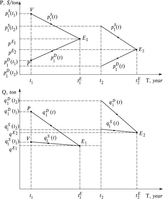
Fig. 1. Trajectory diagram displaying dynamics of the classical two-agent market economy in the one-dimensional economic price space (above) and in the economic quantity space (below). Dimension of time t is year, dimension of the price independent variable P is $/ton, and dimension of the quantity independent variable Q is ton.

A voluntary transaction is accomplished to the mutual satisfaction. Further, the market again is immersed into the state of rest until the next harvest and its display to sale next year at the moment in time of t2. Harvest in this season grew, therefore q1S(t2)> q1S(t1). In this situation, the seller is, obviously, forced to immediately set out the lower starting price, p1S(t2)< p1S(t1), while the buyer, seizing the opportunity, also reduced their price and increased their quantity of grain: p1D(t2)< p1D(t1) and q1D(t2)> q1D(t1). It is natural to expect in this case that the trajectories of the buyer and the seller would be slightly changed, and agreement between the buyer and the seller will be achieved with other parameters than in the previous round of trading.

Conventionally, we will describe the state of the market at every moment in time by the set of real market prices and quantities of real deals which really take place in the market. As we can see from the Fig. 1 real deals occur in the market in our case only at the moments t1E and t2E when the following market equilibrium conditions are valid (points Ei  in Fig. 1):

In this formula, we used several new notions and definitions, whose meanings need explanation. Let us make these explanations in sufficient detail in view of their importance for understanding the following presentation of physical economics. First, in contemporary economic theory, the concept of supply and demand (S&D below) plays one of the central roles. Intuitively, at the qualitative descriptive level, all economists comprehend what this concept means. Complexities and readings appear only in practice with the attempts to give a mathematical treatment to these notions and to develop an adequate method of their calculation and measurement. For this purpose, the various theories contain different mathematical models of S&D that have been developed within the framework. In these theories, differing so-called S&D functions are used to formally define and quantitatively describe S&D.

In this book, we will also repeatedly encounter the various mathematical representations of this concept in different theories, which compose physical economics, namely, classical economy, probability economics, and quantum economy.

Even within the framework of one theory, it is possible to give several formal definitions of S&D functions supplementing each other. For example, within the framework of our two-agent classical economy, we can define total S&D functions as follows:

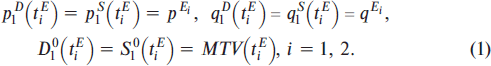
Thus, we have defined at each moment of time t the total demand function of the buyer, D10(t), and the total supply function of the seller, S10(t), as the product of their price and quantity quotations. These functions can be easily depicted in the coordinate system of time and S&D [T, S&D], as it was done in Fig. 2 displaying the so-called S&D diagram. As one would expect, the S&D functions intersect at the equilibrium point E. It is accepted in such cases to indicate that S&D are equal at the equilibrium point. We consider that it is more strictly to say that equilibrium point is that point on the diagram of the trajectories, where these trajectories intersect, i.e., where the price and quantity quotations of the buyer and the seller are equal. But that in this case S&D curves intersect is the simple consequence of their definition equality of prices and quantities at the equilibrium point.

The last observation here concerns a formula for evaluating the volume of trade in the market, MTV(tiE), between the buyer and the seller where they come to a mutual understanding and accomplishment of transaction at the equilibrium point Ei. It is clear that to obtain the trade volume (total value of all the transactions in this case), it is possible to simply multiply the equilibrium values of price and quantity that are derived from the above formula. The dimension of the trade volume is of course a product of the dimensions of price and quantity; in this example this is $. The same is valid for the dimensions of the total S&D, D10(t) and S10(t).

Fig. 2. S&D diagram displaying dynamics of the classical two-agent market economy in the time-S&D functions coordinate system [T, S&D], within the first time interval [t1, t1E].

4.2. The Main Market Rule “Sell all – Buy at all”

Having a method to more or less evaluate the price quantitatively is always advantageous, as it helps us to somewhat predict market prices. Using the main rule of work on the market is used to this end, and this strategic rule of decision making can be briefly formulated as follows: “Sell all – Buy at all”. This main market rule indicates the following different strategies of market actions (action on the market is setting out quotations) for both the seller and the buyer. For the seller this strategy consists in striving to sell all the goods planned to sale at the maximally possible highest prices. Whereas for the buyer this strategy consists in the fact that it will expend all the money planned for the purchase of goods and try to purchase in this case as much as possible at the possible smallest price. Thus, the main market rule leads to the corresponding algorithms of the actions of agents on the markets, which are graphically represented in the form of agents’ trajectories in the pictures. The point of intersection and the respective trade volume in the market, MTV, are easily found with the help of the following mathematical formulas:

It is natural here to name D10(t1) the total demand of buyer at the initial moment of trading. The sense of this quantity is in the fact that this is quantity of resources, planned for the purchase of goods, expressed in the money, although the dimension of this demand is the dimension of money price ($/ton) multiplied by the dimension of quantity (ton). In our case, this is $. We emphasize that, over the course of development of quantitative theory, this is very important in order to draw attention to the dimension of the used quantities and parameters, and to the normalization of the applied functions (see below).

By analogy with classical mechanics, we can treat these prices and quantity functions as the trajectories of movement of the market agents in the two-dimensional economic PQ-space as it was displayed in Fig. 3.

In principle, this representation gives nothing new in comparison with Figs. 1 and 2. Nevertheless, there is one interesting nuance here, in which the similarity of this diagram can be compared to the traditional picture in the conceptual neoclassical model of S&D. We will examine this question below. But let us now focus attention on the following nuances in the picture in Fig. 3. First, it is clearly shown by the arrows, that the buyer and the seller seemingly move towards each other on the price, with the seller reducing it, and the buyer, on the contrary, increasing it. From this, we can reflect on the illustration of normal market negotiation processes. Secondly, usually the quotations of quantities are reduced during the process of negotiations both by the buyer and by the seller. Clearly, all agents want to purchase or to sell a smaller quantity of goods at the compromise market price than at the most desired, presented at the very beginning of trading.

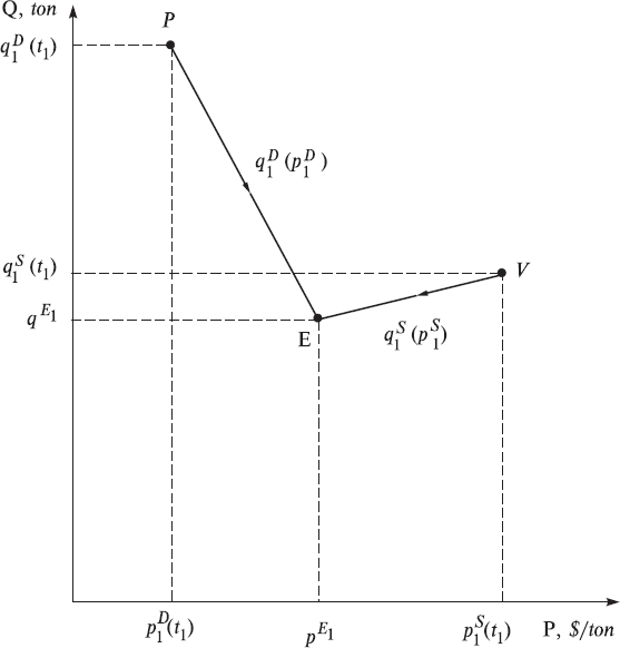
Fig. 3. Dynamics of the classical two-agent market economy in the two-dimensional economic price-quantity space within the first time interval [t1, t1E].

And now we turn from the simplest economy to a more developed economy, in which the farmer and hunter gradually switch from the discrete trade system (one trade per year) to the continuous trade system on the market. Generally speaking, negotiations are conducted continuously and transactions are accomplished continuously, depending on the needs of the buyer and the seller. This would continue for many years. Taking into account this new long-term outlook it is expedient to change somewhat the method of describing the work of the market. Namely, by quotations of a quantity of goods, it is now more convenient to represent a quantity of goods during a specific and reasonable period of time, for example year, if the discussion deals with the long-standing work of the market. In this case the dimension of a quantity would be represented by ton/year. We show in Figs. 4, 5 how it is possible to graphically represent the work of the market over a long span of time. We see that before the establishment of equilibrium at point E, transactions were of course accomplished, but probably did not bring maximum satisfaction to the participants in the market. This would induce agents to continue to search for long-term compromises in prices and quantities. After reaching equilibrium, the volume of trade reaches a maximum, and participants in the market therefore attempt to further support this equilibrium.

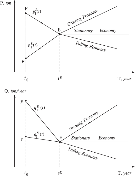
Fig. 4. The classical stationary and non-stationary two-agent market economies in the [T, P] and [T, Q] coordinate systems in the time interval t > tE.

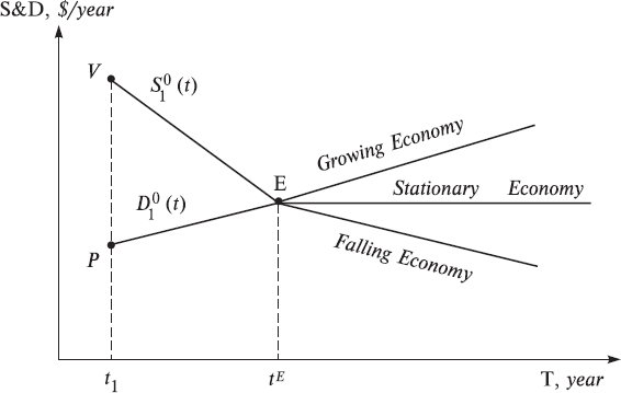
Fig. 5. The classical stationary and non-stationary two-agent market economies in the [T, S&D] – coordinate system.

Here a fork appears in the following theory: – look at Figs. 5 and 6. If quotations cease to change, then the economy converts to a stationary state in which time appears to disappear. This is especially noticeable in Fig. 6, where this sort of stationary state is described by one point, E. We will label the economies in the stationary state simply the stationary economies. But if quotations vary with time, then the economy will be named the time-dependent or simply non-stationary economies. In Figs. 5 and 6 they are represented by two lines, which emanate from the equilibrium point E. If in this case the equilibrium quantity grows, then the economy is a growing one. But if it decreases, then the economy is falling one, which clearly is represented in Fig. 5. As a rule, in such cases, the total S&D behave similarly and this can be easily seen in Fig. 5. Let us note that their dimensions in this model have also changed, now equaling $ · ton/year.

Fig. 6. The classical stationary and non-stationary two-agent market economies in the economic price-quantity space at t > tE.

4.3. The Many-Agent Market Economies

Now we will increase the level of complexity of the classical economies by examining how it is possible to incorporate several buyers and sellers into the theory. It is understandable that each market agent will have its own trajectories in the PQ-space. In principle, they can vary greatly. There is good reason to believe that there is much similarity in the behavior of all buyers in general. The same is valid of course for all sellers. The reason is as follows. There is the intense information exchange on the market, by means of which the coordination of actions is achieved among the buyers, among the sellers, as well as among the buyers and sellers. This coordination is carried out to assist the market in reaching its maximum volume of trade, since it is precisely during the process of trading that the last point is placed in the long process of preliminary business operations: production, financing, logistics, etc. This is exactly what we would have referred to earlier as the social cooperation of the market’s agents. For example, it is natural to expect that all buyers, from one side, and sellers, from other side, behave on the market in approximately the same way, since they all are guided in their behavior on the market by one and the same main rule of work on the market: “Sell all – Buy at all”.

Hence it is possible to draw from the above discussion the following important conclusion: the trajectories of all buyers in the P-space will be close to each other; therefore, the totality of all buyers’ trajectories can be graphically represented in the form of a relatively narrow “pipe”, in which will be plotted the trajectories of all buyers. It is also possible to represent all price trajectories of the buyers by means of a single averaged trajectory, pD(t), which we will do below. We will do the same for the sellers, and their single averaged price trajectory we will designate as pS(t).

We have a completely different situation with the quantity trajectories, since each market agent can have the very different quantities, bearing in mind the fact that the behavior of the buyers’ (sellers’) curves can be relatively similar to each other. Nevertheless, we can establish some regularities in the behavior of the whole market, being guided by common sense and the logical method. Since the quotations of quantities are real in the classical models, we can add them in order to obtain the quantity quotations of the whole market, qD(t) и qS(t). However one should do this separately for the buyers and sellers as follows:

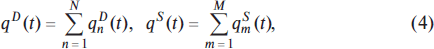
where summing up of quantity quotations is executed formally for the market, which consists of N buyers and M sellers. In this case we understand that for the whole market we can draw all the same pictures as displayed in Figs. 1–6 for the two-agent market. Thus, for instance, we can represent the dynamics of our many-agent market by the help of the following pictures in Fig. 7. In it, the dynamics of many-agent market are depicted at the moment of equilibrium (curves qD(pD) and qS(pS)), as well as dynamics of the stationary economy (point E) and dynamics of the non-stationary growing and falling economies.

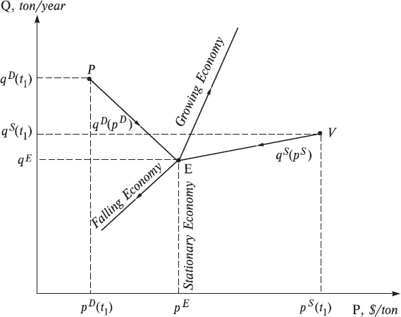
Fig. 7. Dynamics of the many-agent market economy in the price-quantity space. qD(pD) and qS(pS) are quantity trajectories reflecting dynamics of market agents’ quotations in time up to the moment of establishment of the equilibrium and making transactions at the equilibrium price.

4.4. The Classical Economies versus Neoclassical Economies

Let us call attention to the fact that, in Figs. 3 and 6, the quotation curve of the buyer, q1D (pD), has negative slope, and the slope of the quotation curve of the seller, q1S (pS), is positive. This reflects the natural desire of the buyer to purchase more at the lower price, as far as possible, and the natural desire of the seller to sell more at the higher price, as far as possible. Specifically, it is here we reveal the visual similarity of the classical economies to the known neoclassical model of S&D. But the visual similarity of picture in Figs. 3, 6 with the corresponding famous neoclassical picture in the form of two intersected lines of S&D is only formal; economic content in them is entirely different. In classical economies, this is a graphic representation of the real market process (which really occurs on the market at a given instant), while in the neoclassical economies, this picture expresses the planned actions of market agents on the market in the future. Note that in neoclassical economics it is namely the curves qS(pS) and qD(pD) that are called S&D functions. The economic content of these S&D functions can be roughly expressed thus: “the market is by itself, I am by myself”. If one price is on the market, then I purchase (or I sell) one quantity, and if it is another, then will I purchase (or I will sell) another quantity, and so forth. Thus, the market process is completely ignored in the neoclassical economic model. But we know that, in real market life, all market agents participate continuously in the market process, permanently changing price and quantity quotations, since each has made transaction price changes on the market. We will discuss neoclassical models in more detail in other chapters of the book. However, we will now develop an artificial classical economy that will be as similar to the neoclassical model as possible.