Полная версия:
Physical Modeling of Economic Systems

Anatoly Kondratenko
Physical Modeling of Economic Systems
Reviewer:
DSc S.I. Parinov
All rights reserved. No part of the book or whole book may be reproduced or transmitted in any form or by any means without the written permission of the author.
Methods of theoretical physics, classical and quantum mechanics are used to develop classical and quantum models of economies and to derive their equations of motion that describe economy evolution in time, namely, Lagrange and Schrödinger equations correspondingly.
This monograph may seem interesting to everyone who is engaged in research in economics, finance, econophysics or physical economics, as well as to professional investors and stock traders.
PREFACE
This is the first monograph in a series devoted to the development of probabilistic economic theory (Kondratenko, 2005, 2015, 2021). It outlines the fundamental concepts of this theory.
1. Introduction
In the market economy major active players (or agents, or subjects), i.e. buyers and sellers of goods and commodities, behave to a certain extent in a deterministic way thus subordinating their behavior in the market to some strict economic laws. The fact that these laws are of a descriptive nature, and they have not yet been expressed in a precise mathematic language, is not of key importance in this case.
Every rational player or market subject acts in the market in accordance with a strict rule of obtaining maximum profit or benefit or some other criterion of optimality for him or her and in this respect market economic systems resemble physical systems where all players, members, and elements of the system act also in accordance with some principles of maximization.
The main drive of our research is that we assume general possibility to develop dynamic models for relatively simple market economic systems consisting of an economic subsystem or simply an economy with a certain number of buyers and sellers and its external environment with certain interactions between economy agents, and between the economy and environment. In this case, it is supposed that it can be performed by the analogy with the method of developing theoretical models of physical systems consisting of a system of interacting material particles in the external fields or external environment [1, 2]. Moreover, it is assumed that equations of motion derived for physical systems in the physical space are quite a good initial approximation for equations of motion of modeled economic systems in some price space.
Let’s give the following reasons to substantiate such an approach. Let p(t) be a trajectory of movement of the market subject in a price space, in other words, it is price p of a commodity set for by the subject at a moment t. By setting prices this way, buyers and sellers who act as homo negotians (a negotiating man) in a physical modeling aim at maximum satisfaction of their strive for profit, i.e. for such price at which interests of both buyers and sellers and, considering external environment and the whole system in general, are satisfied in an optimal way. It is here that one can see similarity of the movement of economy (described by trajectories p(t)) to the moving of material particles of the physical system (described by trajectories x(t)), which is also subject to a certain principle of maximization. This is what our confidence in conceptual possibility of developing a dynamic theory of economic systems in a price space by the analogy with a dynamic theory of physical systems in physical space is based on. We also admit that in spite of the difference between the qualities of the physical and price spaces along with the qualities of economic and physical systems, the reasonable starting point in the study of economic systems dynamics are equations of motion for a physical prototype, i.e. the type of equations of both systems in their spaces will be the same, though the essence of parameters and potentials in them will be completely different. It is a usual case in physics when one and the same equation describes different systems. For example, the equation of harmonic oscillator describes motion of both simple pendulum and electromagnetic wave. In other words, formal similarity of the equations does not mean equality of the systems which they describe.
In physics a wide experience in calculating physical systems of different degree of complexity with different interaction between members of the system and the system with external environment has been accumulated. It makes sense trying to find a way to use these achievements in finding solutions of economic problems. In case such an activity were successful, there would appear an opportunity of numerical research of the influence of both different internal and external factors on the behavior of each economic agent and on the results of activity of the whole economic system with the help of computer calculations of physical models. Economics (more exactly – theoretical economics) would obtain the most powerful research device the opportunities of which could be compared with the result of the discovery of equations of motion of the physical systems.
The logic of present research is the following. At the first stage of designing a physical model and deriving equations of motion of economic systems from the first principles, or ab initio, we first make all approximations and assumptions required for deriving equations of motion of physical systems in the course of theoretical physics by Landau and Lifshitz [1, 2], then we obtain economic systems equations which are similar to physical systems equations in form and are considered by us as starting or initial approximation for a physical model of the economic system. At the second stage massive model calculations are carried out, their results are compared with experimental or test results, in other words, with the data of empirical economics. At the same time, some optimum values of model parameters and potentials are obtained and the applicability limits of the given initial approximation are estimated. At the third stage suppositions are estimated comparing calculation results and experimental data, and more precise and appropriate optimization principles and corresponding equations of motion are found.
The present book concerns only results of the completed first stage of research at which the main principles of proposed approach to developing physical models of simple market economic systems including economy consisting of several buyers and sellers of certain commodities, and external environment, were developed.
2. Main elements of the physical models
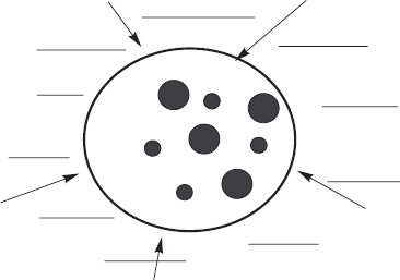
Main elements of our physical models of the economic systems are shown schematically in Fig. 2.1. A large sphere covers a market subsystem or simply economy consisting of active market subjects: buyers who have financial resources and a desire to buy goods or commodities, and sellers who have goods or commodities and a desire to sell them. They are the buyers and sellers who form demand and supply in the market. Small dots inside the sphere denote buyers, big ones denote sellers. Cross-hatched area outside the sphere represents external environment including the state, society and other institutions. The whole economic system is located in some commodity-and-price space which will be discussed below. It is evident that all elements of the system influence each other: buyers compete with each other in the market for commodities; sellers compete with each other for buyers.
The same way buyers and sellers interact with each other thus influencing each other’s behavior. External environment influences all economic agents. In other words, all economic agents are influenced by external environment and interact with each other.
In order to develop a physical model of the economic system, it is necessary to learn to describe exactly in a mathematical way both movement (behavior) of each economic agent, i.e. buyers and sellers, and interaction with each other, and in the end to derive equations of motion which show dynamics or movement, or evolution of the system in time.

Fig. 2.1. Physical model scheme of an economic system: economy consisting of buyers (small dots) and sellers (big dots) which is under the influence of external environment beyond the economy (covered by the sphere).
3. Price space
To show the movement or dynamics of economy it is necessary to introduce a space in which this movement takes place. As an example of such space we choose a commodity-and-price space, or to be more exact simply a price space created by the analogy with a common physical space, where, though, we choose prices pi of the i-th item of commodities as coordinate axes: i = 1 , 2 , … , T, where T is the amount of items of commodities. In case there is one commodity, the space is one-dimensional, i.e. it is represented by one line; the coordinate system for one-dimensional space is shown in Fig. 3.1. The distance between two points in one-dimensional space p′ and p″ is determined as

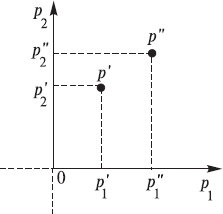
In case there are two commodities, the space is a plane; the coordinate system is represented by two mutually perpendicular lines (see Fig. 3.2), and the distance between two points p′ and p″ is determined as

After the analogy of it we can build a space of any dimension T.
In spite of apparent simplicity, introduction of a price space is of conceptual importance as it allows to describe behavior of market agents in the mathematic language in general. This possibility really exists as setting their own price for commodities any moment of time t is the main function or activity of market agents, and it is, in fact, the main feature or trajectory of agent’s behavior in the market.
It is our main goal to learn to describe these trajectories or connected with them distributions of price probability. It is impossible to do this in a physical space, for example: we can thoroughly describe movement or trajectory of a seller with commodities in physical space, especially if he is in a car or in a spaceship, but it will not have any connection with his attitude to the given commodities and his behavior in this respect (showing his attitude to the commodities by means of his monetary estimation) as an economic agent. Within the problem of describing agents in the market, the role of price as an independent variable, or a coordinate p is considered here as a unique one for market economic systems.

Fig. 3.1. Coordinate system of the one-dimensional price space.

Fig. 3.2. Coordinate system of the two-dimensional price space.
The next step in developing a physical model after selecting a space is selection of a function with the help of which we will try to describe the dynamics of an economy, i.e. movement of buyers and sellers in the price space. Trajectories in coordinate physical space х(t) (classical mechanics), wave functions


4. Classical economy
According to the above-stated plan of actions in this chapter we could confine ourselves to just writing equations of motion analogous to those obtained in classical mechanics. However, we consider it useful to derive a full row of equations and to make additional comments on our actions. First of all, as we have indicated before, we suppose that according to our approach to classical modeling of economic systems every economic agent, homo negotians
Конец ознакомительного фрагмента.
Текст предоставлен ООО «ЛитРес».
Прочитайте эту книгу целиком, купив полную легальную версию на ЛитРес.
Безопасно оплатить книгу можно банковской картой Visa, MasterCard, Maestro, со счета мобильного телефона, с платежного терминала, в салоне МТС или Связной, через PayPal, WebMoney, Яндекс.Деньги, QIWI Кошелек, бонусными картами или другим удобным Вам способом.
Вы ознакомились с фрагментом книги.
Для бесплатного чтения открыта только часть текста.
Приобретайте полный текст книги у нашего партнера:
Полная версия книги
Всего 10 форматов

